Building E-commerce Recommendations with Kumo AI

Building recommendation systems is hard.

In data science, we can spend months wrangling data, training models, and still end up with mediocre results. That's where Kumo AI comes in — it's a service that abstracts away the complexity of building Graph Neural Networks (GNNs) for predictive analytics.

In this article, we'll build a complete e-commerce recommendation engine using real H&M data with 33 million transactions. By the end, we'll have a system that can:

Predict customer lifetime value for the next 30 days
Generate personalized product recommendations
Forecast purchase behavior to identify active customers

The best part? We'll do all this in a couple of hours rather than months.

Why Graph Neural Networks?

Traditional recommendation systems miss the complex relationships between customers, products, and transactions.

GNNs excel here because they naturally model:

Network Effects: How customer preferences influence each other
Temporal Dynamics: Purchase patterns over time (Christmas shopping, summer clothes)
Cold Start Problem: Making predictions for new customers with limited data

Graph structure showing customers connected to transactions connected to products

Kumo was co-founded by one of the pioneers of GNNs and a co-author of the PyG library. Jure Leskovec and the team at Kumo built world-class expertise into the platform, meaning we get top-tier performance without needing deep graph theory knowledge.

Setting Up Kumo

First, install the necessary packages:

python

!pip install -qU \
    "db-dtypes>=1.4.3" \
    "google-auth>=2.40.2" \
    "google-cloud-bigquery>=3.33.0" \
    "kaggle>=1.7.4.5" \
    "kumoai>=2.1.0"

Connecting to Kumo

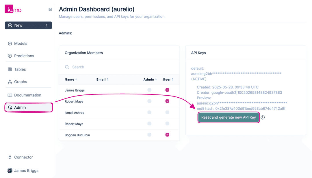
We'll need an API key from our Kumo workspace. Head to the workspace's Admin section to find it.

Kumo AI dashboard API keys section

python

import os
from getpass import getpass
import kumoai

api_key = os.getenv("KUMO_API_KEY") or \
    getpass("Enter your Kumo API key: ")

kumoai.init(url="https://aurelio.kumoai.cloud/api", api_key=api_key)

text

[2025-07-11 15:34:56 - kumoai:196 - INFO] Successfully initialized the Kumo SDK against deployment https://aurelio.kumoai.cloud/api, with log level INFO.

Data Infrastructure

Kumo integrates with our existing data infrastructure. We'll use BigQuery for this tutorial, but S3, Snowflake, and Databricks are also supported.

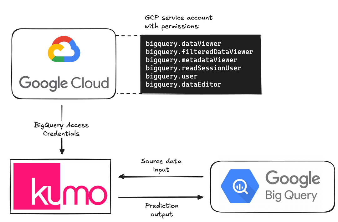
BigQuery Setup

Create a service account in GCP with these permissions:

BigQuery Data Viewer
BigQuery Filtered Data Viewer
BigQuery Metadata Viewer
BigQuery Read Session User
BigQuery User
BigQuery Data Editor

Download the JSON credentials and save as kumo-gcp-creds.json.

BigQuery to Kumo connection flow diagram

python

import json

name = "kumo_intro_live"
project_id = "aurelio-advocacy"  # our GCP project ID
dataset_id = "rel_hm"  # unique dataset ID

with open("kumo-gcp-creds.json", "r") as fp:
    creds = json.loads(fp.read())

connector = kumoai.BigQueryConnector(
    name=name,
    project_id=project_id,
    dataset_id=dataset_id, 
    credentials=creds,
)

This creates our BigQuery connector that Kumo will use to read source data and write predictions.

The H&M Dataset

We're using real H&M transaction data — not a toy dataset.

H&M dataset scale visualization

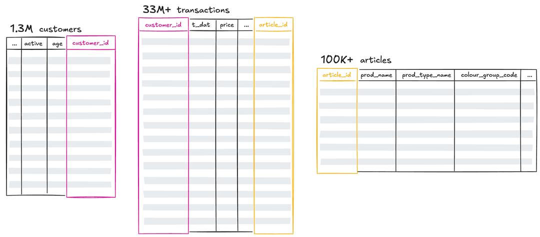
The dataset includes:

1.3M customers with demographics
100K+ products with detailed attributes
33M+ transactions with timestamps

Downloading from Kaggle

First, set up our Kaggle credentials and accept the competition terms.

python

from kaggle.api.kaggle_api_extended import KaggleApi

api = KaggleApi()
api.authenticate()

api.competition_download_files(
    competition="h-and-m-personalized-fashion-recommendations",
    quiet=False
)

This downloads a large zip file (~3.5GB) containing all the competition data.

Extract the CSV files:

python

import zipfile

path = "h-and-m-personalized-fashion-recommendations.zip"

with zipfile.ZipFile(path, "r") as zip_ref:
    file_list = zip_ref.namelist()
    file_list = [f for f in file_list if f.endswith(".csv")]
    for file in file_list:
        zip_ref.extract(file, "hm_data")

We'll have four CSV files:

customers.csv - 1.3M customer records
articles.csv - 100K+ product records
transactions_train.csv - 33M+ transaction records
sample_submission.csv - (we'll skip this one)

Loading into BigQuery

Now we'll push our data to BigQuery where Kumo can access it.

python

from google.cloud import bigquery
from google.oauth2 import service_account

creds_obj = service_account.Credentials.from_service_account_file(
    "kumo-gcp-creds.json",
    scopes=["https://www.googleapis.com/auth/cloud-platform"],
)

client = bigquery.Client(
    credentials=creds_obj,
    project="aurelio-advocacy",
)

Create the dataset:

python

dataset_ref = client.dataset(dataset_id)

try:
    dataset = client.get_dataset(dataset_ref)
    print("Dataset already exists")
except Exception:
    print("Creating dataset...")
    dataset = bigquery.Dataset(dataset_ref)
    dataset.location = "US"
    dataset.description = "H&M Dataset"
    dataset = client.create_dataset(dataset)

Upload each CSV as a table:

python

for file in files[:-1]:  # skip sample_submission.csv
    table_id = file.split("/")[-1].split(".")[0]
    print(f"Pushing {table_id} to BigQuery...")
    table_ref = dataset.table(table_id)
    
    job_config = bigquery.LoadJobConfig(
        write_disposition=bigquery.WriteDisposition.WRITE_TRUNCATE,
        source_format=bigquery.SourceFormat.CSV,
        skip_leading_rows=1,
        autodetect=True,
    )
    
    with open(file, "rb") as f:
        load_job = client.load_table_from_file(
            f, table_ref, job_config=job_config
        )
    load_job.result()
    print(f"Loaded {load_job.output_rows} rows")

text

Pushing customers to BigQuery...
Loaded 1371980 rows
Pushing articles to BigQuery...
Loaded 105542 rows
Pushing transactions_train to BigQuery...
Loaded 31788324 rows

Building Our Graph

With data in BigQuery, we can construct the graph structure for Kumo.

Connect to Source Tables

python

articles_source = connector["articles"]
customers_source = connector["customers"]
transactions_source = connector["transactions_train"]

Let's examine the data structure:

python

articles_source.head()

text

  article_id product_code              prod_name product_type_no product_type_name
0  108775015       108775  Strap top (Yogyakarta)             253          Vest top
1  108775044       108775  Strap top (Yogyakarta)             253          Vest top
2  108775051       108775        Strap top (Salta)             253          Vest top
3  110065001       110065       OP T-shirt (Idro)             306          Bra
4  110065002       110065       OP T-shirt (Idro)             306          Bra

This shows product information including IDs, names, types, colors, and descriptions.

python

customers_source.head(2)

text

                                        customer_id  FN  Active club_member_status fashion_news_frequency  age
0  00000dbac...  NaN     NaN             ACTIVE               NONE   49
1  0000f46a3...  NaN     NaN             ACTIVE               NONE   25

python

transactions_source.head(2)

text

        t_dat                                    customer_id  article_id      price  sales_channel_id
0  2018-09-20  000058a12d5b43e67d225668fa1f8d618c13dc232690b0...  663713001  0.0508305                 2
1  2018-09-20  000058a12d5b43e67d225668fa1f8d618c13dc232690b0...  541518023  0.0305085                 2

Create Kumo Tables

Transform BigQuery tables into Kumo table objects:

python

articles = kumoai.Table.from_source_table(
    source_table=articles_source,
    primary_key="article_id"
).infer_metadata()

customers = kumoai.Table.from_source_table(
    source_table=customers_source,
    primary_key="customer_id"
).infer_metadata()

transactions_train = kumoai.Table.from_source_table(
    source_table=transactions_source,
    time_column="t_dat"
).infer_metadata()

Kumo automatically infers the metadata for each table, including data types and primary/foreign key relationships.

Define the Graph

Connect everything into a graph structure:

python

graph = kumoai.Graph(
    tables={
        "articles": articles,
        "customers": customers,
        "transactions": transactions_train,
    },
    edges=[
        {"src_table": "transactions", "fkey": "customer_id", "dst_table": "customers"},
        {"src_table": "transactions", "fkey": "article_id", "dst_table": "articles"},
    ]
)

graph.validate(verbose=True)

text

[2025-07-11 16:05:42 - kumoai.graph.table:555 - INFO] Table articles is configured correctly.
[2025-07-11 16:05:44 - kumoai.graph.table:555 - INFO] Table customers is configured correctly.
[2025-07-11 16:05:45 - kumoai.graph.table:555 - INFO] Table transactions_train is configured correctly.
[2025-07-11 16:05:47 - kumoai.graph.graph:798 - INFO] Graph is configured correctly.

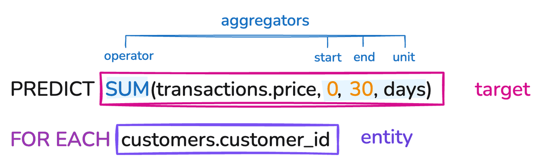
Predictive Query Language (PQL)

Here's where Kumo shines.

Instead of writing complex neural network code, we describe predictions using SQL-like PQL.

Use Case 1: Customer Lifetime Value

Predict total revenue per customer over the next 30 days:

PQL syntax for customer value prediction

python

pquery = kumoai.PredictiveQuery(
    graph=graph,
    query=(
        "PREDICT SUM(transactions.price, 0, 30, days)\n"
        "FOR EACH customers.customer_id\n"
    )
)

pquery.validate(verbose=True)

text

[2025-07-11 16:12:47 - kumoai.pquery.predictive_query:211 - INFO] Query PREDICT SUM(transactions.price, 0, 30, days)
FOR EACH customers.customer_id
 is configured correctly.

Get Kumo's recommended model parameters:

python

model_plan = pquery.suggest_model_plan()
model_plan

This returns a comprehensive model plan with:

Training parameters (learning rates, batch sizes, epochs)
GNN architecture details (channels, aggregation methods)
Optimization settings (loss functions, weight decay)

Start training:

python

trainer = kumoai.Trainer(model_plan=model_plan)
training_job = trainer.fit(
    graph=graph,
    train_table=pquery.generate_training_table(non_blocking=True),
    non_blocking=True,
)

text

[2025-07-11 16:17:57 - kumoai.graph.graph:394 - INFO] Graph snapshot created.
[2025-07-11 16:18:00 - kumoai.graph.graph:462 - WARNING] Graph snapshot already exists, will not be refreshed.

Use Case 2: Product Recommendations

Predict top 10 products each customer will likely buy:

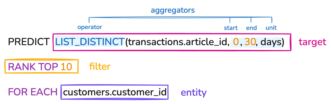
PQL syntax for product recommendations

python

purchase_pquery = kumoai.PredictiveQuery(
    graph=graph,
    query=(
        "PREDICT LIST_DISTINCT(transactions.article_id, 0, 30)\n"
        "RANK TOP 10\n"
        "FOR EACH customers.customer_id\n"
    )
)

purchase_pquery.validate(verbose=True)

text

[2025-07-11 16:23:59 - kumoai.pquery.predictive_query:211 - INFO] Query PREDICT LIST_DISTINCT(transactions.article_id, 0, 30)
RANK TOP 10
FOR EACH customers.customer_id
 is configured correctly.

Train the model:

python

model_plan = purchase_pquery.suggest_model_plan()
purchase_trainer = kumoai.Trainer(model_plan=model_plan)
purchase_training_job = purchase_trainer.fit(
    graph=graph,
    train_table=purchase_pquery.generate_training_table(non_blocking=True),
    non_blocking=True,
)

Use Case 3: Purchase Volume

Predict transaction count for recently active customers:

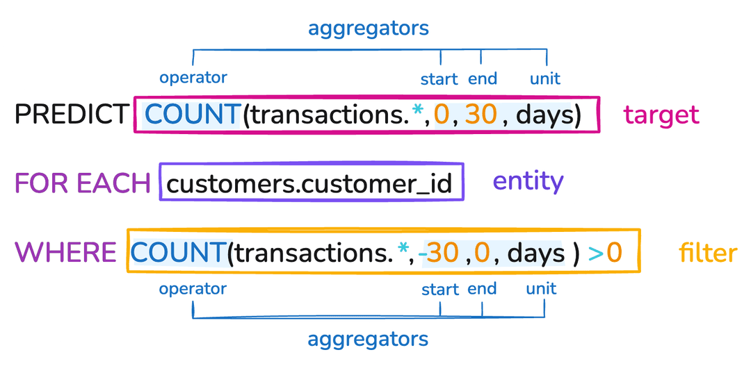
PQL syntax for transaction predictions

python

transactions_pquery = kumoai.PredictiveQuery(
    graph=graph,
    query=(
        "PREDICT COUNT(transactions.*, 0, 30)\n"
        "FOR EACH customers.customer_id\n"
        "WHERE COUNT(transactions.*, -30, 0) > 0\n"
    )
)

transactions_pquery.validate(verbose=True)

text

[2025-07-11 16:27:30 - kumoai.pquery.predictive_query:211 - INFO] Query PREDICT COUNT(transactions.*, 0, 30)
FOR EACH customers.customer_id
WHERE COUNT(transactions.*, -30, 0) > 0
 is configured correctly.

The WHERE clause filters for customers active in the past 30 days, reducing prediction scope.

Making Predictions

Once models finish training (40-60 minutes), generate predictions:

python

# Check training status
training_job.status()

Customer Value Predictions

python

from kumoai.artifact_export.config import OutputConfig

predictions = trainer.predict(
    graph=graph,
    prediction_table=pquery.generate_prediction_table(non_blocking=True),
    output_config=OutputConfig(
        output_types={"predictions"},  
        output_connector=connector,
        output_table_name="SUM_TRANSACTIONS_PRED",
    ),
    training_job_id=training_job.id,
    non_blocking=True,
)

text

[2025-07-11 18:12:51 - kumoai.trainer.trainer:418 - WARNING] Prediction produced the following warnings: 
For the optimal experience, it is recommended for output tables to only contain uppercase characters, numbers, and underscores

Product Recommendations

For ranking predictions, specify how many results per entity:

python

purchase_predictions = purchase_trainer.predict(
    graph=graph,
    prediction_table=purchase_pquery.generate_prediction_table(non_blocking=True),
    num_classes_to_return=10,  # top 10 products
    output_config=OutputConfig(
        output_types={"predictions"},
        output_connector=connector,
        output_table_name="PURCHASE_PRED",
    ),
    training_job_id=purchase_training_job.id,
    non_blocking=True,
)

Transaction Volume

python

transactions_predictions = transactions_trainer.predict(
    graph=graph,
    prediction_table=transactions_pquery.generate_prediction_table(non_blocking=True),
    output_config=OutputConfig(
        output_types={"predictions"},
        output_connector=connector,
        output_table_name="TRANSACTIONS_PRED",
    ),
    training_job_id=transactions_training_job.id,
    non_blocking=True,
)

These prediction jobs will write results to new tables in BigQuery with the suffix _predictions.

Analyzing Results

Kumo writes predictions back to BigQuery. Let's analyze them.

Top Value Customers

python

query = f"""
SELECT * FROM {dataset_id}.SUM_TRANSACTIONS_PRED_predictions
ORDER BY TARGET_PRED DESC
LIMIT 5
"""

client.query(query).to_dataframe()

text

                                            ENTITY  TARGET_PRED
0  63d4ee9c373b7ec52fd03b319faf53f3f1f24763d8a3ac...     0.668505
1  f69cf6fca69045a8259f9554e318e00fbf5e8e758e88b1...     0.657948
2  be96311f48cf1049e0da065ab322fada512ee88486c371...     0.647882
3  203785d96661d87a84718e998664c1169f43aa21b677a1...     0.643395
4  17d6270f6f81ad1f7e5a1cb7ed8edb54bc00d0d5c2cde6...     0.640910

Finding Customer Preferences

Let's identify our most valuable customers and their preferences:

python

valuable_customers = f"""
SELECT cust.*, trans.target_pred AS score FROM {dataset_id}.customers cust
INNER JOIN (
    SELECT entity, target_pred FROM {dataset_id}.SUM_TRANSACTIONS_PRED_predictions
    ORDER BY target_pred DESC
    LIMIT 30
) trans ON cust.customer_id = trans.entity
"""

top_customers = client.query(valuable_customers + ";").result().to_dataframe()
top_customers.head()

text

                                       customer_id   FN  Active club_member_status fashion_news_frequency  age     score
0  e9c27cf3d00e7bb6a27f395a01d01fbe6328901afdb645...  NaN     NaN             ACTIVE                   NONE   22  0.599846
1  ceb037bfdab35cdd507685b20648829ddc0d92c8e02e2f...  NaN     NaN             ACTIVE                   NONE   24  0.621152
2  d8c54f5ca6421ba8c5d7631ebdf7a5b67ccf2dce4b859c...  NaN     NaN             ACTIVE                   NONE   25  0.585189
3  8c40103139dd4b93163fa25a536cac2351ebb5936700cb...  1.0     1.0             ACTIVE              Regularly   25  0.575516
4  d1bbee89e5364ecdb031e2b2f4be3509029d007eac99a2...  1.0     1.0             ACTIVE              Regularly   37  0.610632

Now see what the top customer will likely buy:

python

product_recs = f"""
SELECT
    pred.entity AS customer_id,
    pred.score AS score,
    art.*
FROM {dataset_id}.PURCHASE_PRED_predictions pred
INNER JOIN {dataset_id}.articles art ON pred.class = art.article_id
INNER JOIN {dataset_id}.customers cust ON pred.entity = cust.customer_id
WHERE cust.customer_id = '{top_customers.customer_id[0]}'
"""

top_cust_recs = client.query(product_recs).result().to_dataframe()
top_cust_recs

text

                                       customer_id     score  article_id product_code               prod_name product_type_no product_type_name
0  e9c27cf3d00e7bb6a27f395a01d01fbe6328901afdb645...  7.167438   787285001       787285                   Magic             265             Dress
1  e9c27cf3d00e7bb6a27f395a01d01fbe6328901afdb645...  7.023399   859957001       859957      LE Good Ada Dress             265             Dress
2  e9c27cf3d00e7bb6a27f395a01d01fbe6328901afdb645...  6.783765   758381002       758381            Twist fancy              92    Heeled sandals
3  e9c27cf3d00e7bb6a27f395a01d01fbe6328901afdb645...  6.890747   935635002       935635   LUCKY TIE NECK SHIRT             259             Shirt
4  e9c27cf3d00e7bb6a27f395a01d01fbe6328901afdb645...  6.762956   787285003       787285                   Magic             265             Dress
5  e9c27cf3d00e7bb6a27f395a01d01fbe6328901afdb645...  7.849483   904625001       904625      Pax HW PU Joggers             272          Trousers
6  e9c27cf3d00e7bb6a27f395a01d01fbe6328901afdb645...  7.308242   918212001       918212           ED Uma dress             265             Dress
7  e9c27cf3d00e7bb6a27f395a01d01fbe6328901afdb645...  7.370093   787285005       787285                   Magic             265             Dress
8  e9c27cf3d00e7bb6a27f395a01d01fbe6328901afdb645...  7.245024   814980001       814980          Alabama Dress             265             Dress
9  e9c27cf3d00e7bb6a27f395a01d01fbe6328901afdb645...  6.791434   835247001       835247              Supernova             265             Dress

This customer clearly loves dresses — 7 out of 10 recommendations are dresses!

Purchase Volume Analysis

Finally, predict transaction volume for valuable customers:

python

predicted_volume = f"""
SELECT cust.customer_id, trans.target_pred
FROM ({valuable_customers}) cust
INNER JOIN {dataset_id}.TRANSACTIONS_PRED_predictions trans 
ON cust.customer_id = trans.entity
"""

cust_volume = client.query(predicted_volume).result().to_dataframe()
cust_volume.head()

text

                                        customer_id  target_pred
0  2cabdc6101018f8cea44310343769715049befed47caa9...    19.226614
1  77db96923d20d40532eba0020b55cd91eb51358885c2d6...    10.042411
2  062234bcfa5875d71069215348a11f100aa15edd540868...    12.537105
3  2baed3260d6a0c2f23737d09b68d30eff348eb8ec428e0...    15.382269
4  788785852eddb5874f924603105f315d69571b3e5180f3...    10.424101

Our top valuable customers are predicted to make between 10-20 transactions in the next 30 days.

What Makes This Powerful

Building a pipeline like this can take weeks or months — data wrangling, model training (and retraining again and again), followed by analytics can easily become a long-running project. As we demonstrated here,we can build the same pipeline in hours with Kumo — and the results are likely better than what many of us can achieve solo.

This democratizes advanced analytics. We don't need deep GNN expertise to provide world-class insights to complex data and business questions — we use Kumo.